Spatial and Spatio-Temporal Models

Overview

When small areas are geographic units (such as counties, regencies, or districts), spatial correlation frequently occurs: neighboring areas tend to have more similar outcomes than distant ones. Furthermore, when surveys are repeated over multiple years, temporal correlation between time periods is also present.

fastsae provides specialized, high-performance implementations for both: 1. Spatial Fay-Herriot (eblup_sfh): Simultaneous Autoregressive SAR(1) random effects. 2. Spatio-Temporal Fay-Herriot (eblup_stfh): Combined spatial SAR(1) and temporal AR(1) random effects.

---

1. Spatial Fay-Herriot Model (eblup_sfh)

Model Formulation

The Spatial Fay-Herriot model (Pratesi & Salvati, 2008) models area random effects using a Simultaneous Autoregressive (SAR(1)) process:

$$y = X\beta + u + e$$

$$u = \rho_1 W u + \epsilon_1 \implies u = (I - \rho_1 W)^{-1} \epsilon_1$$

where: - $W$ is a known row-standardized spatial proximity matrix ($D \times D$). - $\rho_1 \in (-1, 1)$ is the spatial autoregressive parameter. - $\epsilon_1 \sim N(0, \sigma_{u1}^2 I_D)$ is independent innovation noise. - $e \sim N(0, V_e)$ is sampling error with diagonal matrix $V_e = \text{diag}(D_1, \dots, D_D)$.

Fitting the Model

library(fastsae)
data("mys")
data("mys_proxmat")

# Fit Spatial Fay-Herriot model with REML
fit_sfh <- eblup_sfh(
  formula = y ~ x1 + x2 + x3,
  vardir = ~vardir,
  data = mys,
  W = mys_proxmat,
  method = "REML",
  print_result = FALSE
)

summary(fit_sfh)
#> 
#> ── Summary of fastsae Fit ──────────────────────────────────────────────────────
#> Call :
#> eblup_sfh(formula = y ~ x1 + x2 + x3, vardir = ~vardir, data = mys, method =
#> "REML", W = mys_proxmat, print_result = FALSE)
#> 
#> ✔ Convergence: Yes (in 18 iterations)
#> Model: Spatial Fay-Herriot (Area-level SAR)
#> Method: REML
#> 
#> Variance & Correlation Components:
#>  parameter   estimate std.error
#>   sigma2_u  0.9892261 0.4797447
#>        rho -1.0000000        NA
#> rho (spatial): -1 
#> 
#> Coefficients:
#>                   beta  std.error     zvalue pvalue
#> (Intercept)  3.2570714  0.6265689  5.1982651 0.0000
#> x1          -0.0020340  0.0080925 -0.2513457 0.8015
#> x2           0.0568516  0.0525488  1.0818827 0.2793
#> x3           0.0252179  0.0497283  0.5071123 0.6121
#> 
#> Goodness of Fit:
#> loglikelihood           AIC           BIC 
#>     -62.58874     137.17748     145.97189 
#> 
#> EBLUP Summary Statistics:
#>       mse              rse        
#>  Min.   :0.1966   Min.   : 9.384  
#>  1st Qu.:0.5897   1st Qu.:13.643  
#>  Median :0.8169   Median :19.046  
#>  Mean   :1.0420   Mean   :22.242  
#>  3rd Qu.:1.4214   3rd Qu.:27.305  
#>  Max.   :2.1610   Max.   :46.894

Unsampled Domains and Spatial Kriging

A major advantage of eblup_sfh in fastsae is its automatic handling of unsampled domains (domains with y = NA). Instead of throwing an error or requiring manual subsetting, eblup_sfh automatically performs full-spatial kriging:

# Count sampled vs unsampled domains
table(is.na(mys$y))
#> 
#> FALSE  TRUE 
#>    32    10

# Inspect estimates for unsampled domains
head(fit_sfh$df_eblup[is.na(mys$y), ])
#>    domain  y vardir    eblup random_effect      mse      rse
#> 21     21 NA      0 4.136624    0.33273263 1.773635 32.19482
#> 25     25 NA      0 3.666578   -0.63352730 1.606281 34.56606
#> 26     26 NA      0 6.293404    0.82251711 1.962186 22.25792
#> 27     27 NA      0 5.185438    0.66260236 1.879788 26.44046
#> 28     28 NA      0 5.159499   -0.02771458 1.448608 23.32748
#> 34     34 NA      0 3.834916    0.17166576 1.587847 32.85856

For unsampled areas, prediction borrows strength from both the regression synthetic component $x_d^\top \hat{\beta}$ and spatial proximity to neighboring sampled areas through $(I - \hat{\rho}_1 W)^{-1}$.

Multi-Threaded Bootstrap MSE

In addition to analytical Prasad-Rao style MSE, eblup_sfh supports multi-threaded OpenMP bootstrap MSE estimation:

• Parametric Bootstrap (mse_type = "pbmse")
• Non-Parametric Bootstrap (mse_type = "npbmse")

fit_sfh_pb <- eblup_sfh(
  formula = y ~ x1 + x2 + x3,
  vardir = ~vardir,
  data = mys,
  W = mys_proxmat,
  mse_type = "pbmse",
  B = 50,
  n_threads = 2,
  seed = 123,
  print_result = FALSE
)
#> ℹ 10 unsampled domain(s) detected. Bootstrap MSE (pbmse) is computed for the 32 sampled domain(s); unsampled domain(s) get a full-spatial synthetic (kriging) prediction and analytical MSE instead.

head(fit_sfh_pb$df_eblup[, c("domain", "y", "eblup", "mse", "mse_pb", "mse_pbbc")])
#>   domain        y    eblup       mse    mse_pb  mse_pbbc
#> 1      1 8.359527 7.535193 0.4999462 0.5854030 0.5806763
#> 2      2 7.599650 6.564385 0.5831410 0.7066187 0.6551951
#> 3      3 5.514137 5.109460 0.6095214 0.7523068 0.6805248
#> 4      4 3.869326 4.273391 0.5018535 0.5752400 0.5553161
#> 5      5 6.305063 6.791422 0.7644430 0.7612421 0.8819870
#> 6      6 3.926807 4.016701 0.3398919 0.3751907 0.3681698

---

2. Spatio-Temporal Fay-Herriot Model (eblup_stfh)

Model Formulation

The Spatio-Temporal model (Marhuenda, Molina, & Morales, 2013) combines spatial correlation and temporal autoregression for $D$ areas over $T$ time periods. The panel does not need to be complete: cells without a direct estimate are predicted (see below).

$$y_{dt} = x_{dt}^\top \beta + u_{1d} + u_{2dt} + e_{dt}$$

where: - $u_1 = (u_{11}, \dots, u_{1D})^\top$ captures static spatial effects: $u_1 = \rho_1 W u_1 + \epsilon_1$. - $u_{2d} = (u_{2d1}, \dots, u_{2dT})^\top$ captures dynamic temporal effects for area $d$: $u_{2dt} = \rho_2 u_{2d,t-1} + \epsilon_{2dt}$. - $e_{dt} \sim \text{ind. } N(0, D_{dt})$ are sampling errors.

The model is defined on the full $D \times T$ grid: $u_1$ on all domains of $W$, $u_2$ on all periods.

Fitting the Spatio-Temporal Model

data("mys_panel")

# 42 domains x 11 years; y is NA for the two domains that are never sampled
table(sampled = !is.na(mys_panel$y))
#> sampled
#> FALSE  TRUE 
#>    22   440

# Fit Spatio-Temporal model with the analytical MSE, on the full panel and full W
fit_stfh <- eblup_stfh(
  formula = y ~ x1 + x2 + x3,
  data = mys_panel,
  vardir = ~vardir,
  domain = ~area,
  time = ~year,
  W = mys_proxmat,
  model = "ST",
  mse_type = "analytical",
  print_result = FALSE
)

summary(fit_stfh)
#> 
#> ── Summary of fastsae Fit ──────────────────────────────────────────────────────
#> Call :
#> eblup_stfh(formula = y ~ x1 + x2 + x3, vardir = ~vardir, data = mys_panel,
#> domain = ~area, time = ~year, W = mys_proxmat, model = "ST", mse_type =
#> "analytical", print_result = FALSE)
#> 
#> ✔ Convergence: Yes (in 16 iterations)
#> Model: Spatio-Temporal Fay-Herriot (SAR + AR(1) time effects)
#> Method: REML
#> Cells without a direct estimate: 22 of 462 (predicted from the model)
#> 
#> Variance & Correlation Components:
#>       estimate   std.error
#>   1.8250368492 0.790026019
#>  -0.9990000000          NA
#>   0.0005145706 0.001444823
#>   0.9990000000          NA
#> 
#> Coefficients:
#>                    beta   std.error      zvalue pvalue
#> (Intercept)  4.39878365  0.44921728  9.79210703 0.0000
#> x1          -0.00068256  0.00597669 -0.11420395 0.9091
#> x2           0.02595246  0.02772502  0.93606644 0.3492
#> x3           0.01695061  0.02570240  0.65949541 0.5096
#> 
#> Goodness of Fit:
#> loglikelihood           AIC           BIC 
#>     -597.2793     1210.5587     1243.2529 
#> 
#> EBLUP Summary Statistics:
#>       mse               rse          
#>  Min.   :0.01994   Min.   :   2.912  
#>  1st Qu.:0.07623   1st Qu.:   5.056  
#>  Median :0.10770   Median :   5.980  
#>  Mean   :0.26423   Mean   :  24.908  
#>  3rd Qu.:0.16075   3rd Qu.:   9.470  
#>  Max.   :2.63652   Max.   :2680.093

The estimated variance and correlation components include: - sigma21: Spatial random effect variance ($\sigma_{u1}^2$). - rho1: Spatial autocorrelation ($\rho_1$). - sigma22: Temporal random effect variance ($\sigma_{u2}^2$). - rho2: Temporal AR(1) autoregression coefficient ($\rho_2$).

The analytical MSE is $g_1 + g_2 + 2 g_3 - g_4$ (Prasad-Rao type, with the exact derivative of the EBLUP in $g_3$ and the curvature term $g_4$ for the nonlinear $\rho_1$, $\rho_2$); the components are returned as fit_stfh$g1, …, fit_stfh$g4. A parametric bootstrap MSE is available with mse_type = "bootstrap" (and B, seed).

Unsampled Domains and Missing Periods

Rows whose response is NA are kept and predicted, as long as the auxiliary variables are known there. The variance components are estimated from the sampled cells only (the marginal likelihood with the missing cells integrated out), and each missing cell gets the best linear unbiased predictor given the sampled data (Saei & Chambers, 2005; Benedetti et al., 2024):

• a missing period of a sampled domain borrows from the other periods of that domain (AR(1) correlation) and from the neighbouring domains (SAR);
• a domain that is never sampled is predicted from its neighbours only (spatial kriging), so W must keep it.

est <- fit_stfh$df_eblup
# Cells predicted without a direct estimate
head(est[!est$sampled, c("domain", "time", "eblup", "mse", "rse")])
#>     domain time    eblup      mse      rse
#> 21      21 2016 6.137783 2.626182 26.40285
#> 25      25 2016 3.369663 2.557295 47.45741
#> 63      21 2017 6.148986 2.619596 26.32168
#> 67      25 2017 3.359054 2.572143 47.74530
#> 105     21 2018 6.142760 2.625602 26.37855
#> 109     25 2018 3.319488 2.595463 48.53291

# Their MSE is larger: no direct estimate, only borrowed strength
tapply(est$mse, ifelse(est$sampled, "sampled", "unsampled"), median)
#>   sampled unsampled 
#> 0.1061676 2.6167041

For these cells the analytical MSE is $g_1 + g_2 + g_3$ ($g_3$ from the exact derivative of the predictor in the variance components); the bootstrap generates the random effects on the full grid and covers every cell too.

---

3. Comparing Models with autoplot

You can directly compare EBLUP estimates and uncertainty across different models using autoplot():

# Compare Fay-Herriot vs Spatial Fay-Herriot
fit_fh <- eblup_fh(y ~ x1 + x2 + x3, vardir = ~vardir, data = na.omit(mys), print_result = FALSE)
W_clean <- mys_proxmat[!is.na(mys$y), !is.na(mys$y)]
fit_sfh_clean <- eblup_sfh(y ~ x1 + x2 + x3, vardir = ~vardir, data = na.omit(mys), W = W_clean, print_result = FALSE)
#> Warning: `W` is not row-standardised: some rows do not sum to 1.
#> ℹ The SAR model with rho in (-1, 1) assumes rows summing to 1; use `W /
#>   rowSums(W)` or `create_weights(style = "W")`.

autoplot(list("Standard FH" = fit_fh, "Spatial FH" = fit_sfh_clean), type = "comparison")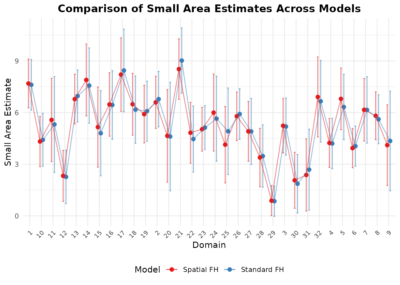

---

4. Bayesian Spatio-Temporal Modeling (hb_area)

In addition to frequentist C++ EBLUP implementations (eblup_sfh and eblup_stfh), fastsae provides hb_area() for Bayesian spatio-temporal modeling powered by INLA. This supports: - Bounded proportions via Beta regression (matching tipsae) - Discrete counts via Poisson and Negative Binomial regression - Binary aggregates via Binomial regression - Flexible space-time structures including domain-specific random walks, separable dynamic fields, and Knorr-Held Types I–IV.

For full details and a case study on Italian poverty data, see the vignette Bayesian Area-Level Small Area Estimation with INLA.

---

References

• Benedetti, R., Piersimoni, F., Pratesi, M., Salvati, N., & Suesse, T. (2024). Handling out-of-sample areas to estimate the unemployment rate at local labour market areas in Italy. International Statistical Review. https://doi.org/10.1111/insr.12596
• Marhuenda, Y., Molina, I., & Morales, D. (2013). Small area estimation with spatio-temporal Fay-Herriot models. Computational Statistics & Data Analysis, 58, 308–325.
• Pratesi, M., & Salvati, N. (2008). Small area estimation: The EBLUP estimator based on spatially correlated random area effects. Statistical Methods & Applications, 17(1), 113–141.
• Saei, A., & Chambers, R. (2005). Out of sample estimation for small areas using area level data. Southampton Statistical Sciences Research Institute, Methodology Working Paper M05/11.