
Unit-Level Estimation with Battese-Harter-Fuller
Source:vignettes/unit-level-bhf.Rmd
unit-level-bhf.RmdOverview
Unlike area-level models that aggregate data prior to modeling, unit-level models operate directly on individual survey unit records (e.g., households, farms, or persons) while linking them to population auxiliary aggregates (e.g., census means or satellite imagery).
The fastsae package implements the nested error
regression model of Battese, Harter, and Fuller (1988) via
eblup_bhf(), providing fast estimation and parallel
parametric bootstrap MSE. hb_unit() fits the same model as
a hierarchical Bayes model with INLA (see the last section).
Model Formulation
For individual unit () in small area ():
where: - is the area-specific random effect. - is the unit-level error variance. - and are mutually independent.
The small area population mean is estimated by:
where: - is the known population mean vector of auxiliary variables for domain . - and are the sample means for domain . - is the shrinkage ratio.
Step-by-Step Example
1. Data Preparation
We use the classic cornsoybean dataset, reporting corn
crop hectares per segment in 12 Iowa counties:
library(fastsae)
data("cornsoybean")
data("cornsoybeanmeans")

# Align column names for population auxiliary means
df_pop <- cornsoybeanmeans
names(df_pop)[names(df_pop) == "MeanCornPixPerSeg"] <- "CornPix"
names(df_pop)[names(df_pop) == "MeanSoyBeansPixPerSeg"] <- "SoyBeansPix"
names(df_pop)[names(df_pop) == "CountyIndex"] <- "County"

head(cornsoybean)
#>   County CornHec SoyBeansHec CornPix SoyBeansPix
#> 1      1  165.76        8.09     374          55
#> 2      2   96.32      106.03     209         218
#> 3      3   76.08      103.60     253         250
#> 4      4  185.35        6.47     432          96
#> 5      4  116.43       63.82     367         178
#> 6      5  162.08       43.50     361         137
head(df_pop)
#>   County CountyName SampSegments PopnSegments CornPix SoyBeansPix
#> 1      1 CerroGordo            1          545  295.29      189.70
#> 2      2   Hamilton            1          566  300.40      196.65
#> 3      3      Worth            1          394  289.60      205.28
#> 4      4   Humboldt            2          424  290.74      220.22
#> 5      5   Franklin            3          564  318.21      188.06
#> 6      6 Pocahontas            3          570  257.17      247.13
2. Fit BHF Model with Bootstrap MSE
We fit the model using eblup_bhf(). The domain-level
Mean Squared Error (MSE) is estimated by parametric bootstrap
(mse_type = "bootstrap", the default;
mse_type = "none" skips it):
fit_bhf <- eblup_bhf(
  formula = CornHec ~ CornPix + SoyBeansPix,
  unit_data = cornsoybean,
  Xpop = df_pop,
  domain_var = "County",
  popsize_var = "PopnSegments",
  method = "REML",
  mse_type = "bootstrap",
  B = 50,
  seed = 123,
  print_result = FALSE
)

summary(fit_bhf)
#>
#> ── Summary of fastsae Fit ──────────────────────────────────────────────────────
#> Call :
#> eblup_bhf(formula = CornHec ~ CornPix + SoyBeansPix, unit_data = cornsoybean,
#> Xpop = df_pop, domain_var = "County", popsize_var = "PopnSegments", method =
#> "REML", B = 50, mse_type = "bootstrap", seed = 123, print_result = FALSE)
#>
#> ✔ Convergence: Yes (in - iterations)
#> Model: Battese-Harter-Fuller (Unit-level)
#>
#> Variance Components:
#> sigma2_u: 63.31489
#>
#> Coefficients:
#>                  beta std.error    zvalue pvalue
#> (Intercept) 17.963979 30.974505  0.579960 0.5619
#> CornPix      0.366335  0.064959  5.639511 0.0000
#> SoyBeansPix -0.030364  0.067576 -0.449327 0.6532
#>
#> Goodness of Fit:
#> loglikelihood           AIC           BIC
#>     -159.2759      328.5517      336.6063
#>
#> EBLUP Summary Statistics:
#>       mse             rse
#>  Min.   :24.89   Min.   :4.039
#>  1st Qu.:36.74   1st Qu.:4.838
#>  Median :46.45   Median :5.816
#>  Mean   :49.96   Mean   :5.839
#>  3rd Qu.:62.20   3rd Qu.:6.849
#>  Max.   :81.65   Max.   :7.921
3. Inspect Domain Estimates
The resulting df_eblup data frame contains the domain
estimates along with sample size, MSE, and Relative Standard Error
(RSE):
head(fit_bhf$df_eblup)
#>   domain    eblup samp_size      mse      rse
#> 1      1 122.5825         1 81.64650 7.371235
#> 2      2 123.5274         1 69.94383 6.770354
#> 3      3 113.0343         1 80.17283 7.921429
#> 4      4 114.9901         2 52.75789 6.316599
#> 5      5 137.2660         3 32.60240 4.159698
#> 6      6 108.9807         3 59.61422 7.084763
4. Visualizing Results with autoplot
For unit-level models, domain uncertainty and model comparisons can
be displayed with autoplot():
# Plot MSE across counties
autoplot(fit_bhf, type = "mse")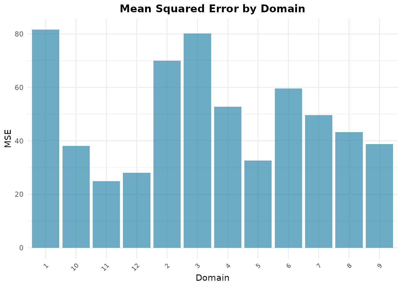
# Plot EBLUP estimates with confidence intervals
autoplot(fit_bhf, type = "comparison")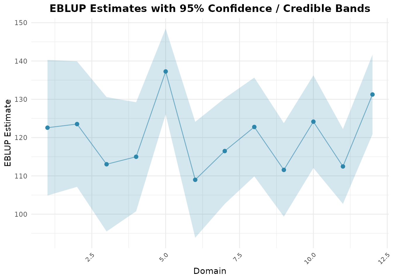
Hierarchical Bayes with hb_unit()
hb_unit() fits the nested error model with INLA and
returns posterior means, standard deviations and credible intervals of
the county means. It needs the INLA package, which is
not on CRAN (https://www.r-inla.org/download/); the chunks below are
only run when INLA is installed. The arguments are those of
eblup_bhf():
fit_hbu <- hb_unit(
  CornHec ~ CornPix + SoyBeansPix,
  unit_data = cornsoybean,
  Xpop = df_pop,
  domain_var = "County",
  popsize_var = "PopnSegments",
  print_result = FALSE
)

head(fit_hbu$df_hb[, c("domain", "samp_size", "hb", "sd", "ci_lower", "ci_upper")])
#>   domain samp_size       hb       sd  ci_lower ci_upper
#> 1      1         1 122.7198 8.782060 105.50695 139.9326
#> 2      2         1 123.6712 8.630843 106.75478 140.5877
#> 3      3         1 112.3976 9.450425  93.87474 130.9204
#> 4      4         2 114.8463 7.925441  99.31239 130.3801
#> 5      5         3 136.6270 8.575491 119.81909 153.4350
#> 6      6         3 108.7228 7.349307  94.31820 123.1275
County by county, the posterior means are close to the EBLUP:
data.frame(
  County = fit_bhf$df_eblup$domain,
  n = fit_bhf$df_eblup$samp_size,
  eblup = round(fit_bhf$df_eblup$eblup, 1),
  hb = round(fit_hbu$df_hb$hb, 1),
  rmse_eblup = round(sqrt(fit_bhf$df_eblup$mse), 1),
  sd_hb = round(fit_hbu$df_hb$sd, 1)
)
#>    County n eblup    hb rmse_eblup sd_hb
#> 1       1 1 122.6 122.7        9.0   8.8
#> 2       2 1 123.5 123.7        8.4   8.6
#> 3       3 1 113.0 112.4        9.0   9.5
#> 4       4 2 115.0 114.8        7.3   7.9
#> 5       5 3 137.3 136.6        5.7   8.6
#> 6       6 3 109.0 108.7        7.7   7.3
#> 7       7 3 116.5 116.6        7.0   6.9
#> 8       8 3 122.8 122.6        6.6   6.9
#> 9       9 4 111.6 111.0        6.2   6.9
#> 10     10 5 124.2 124.4        6.2   6.0
#> 11     11 5 112.5 113.4        5.0   7.2
#> 12     12 6 131.3 131.3        5.3   5.7
The two sets of estimates differ by about 1 hectare at most (under 1%
of the county means). The bootstrap root MSE and the posterior SD are
different quantities; here the SDs are larger in 10 of the 12 counties
(by up to half in counties 5 and 11), and with B = 50 the
bootstrap MSE is itself noisy.
The prior of
is half-normal with the scale of the unit responses (see
vignette("hb-priors")). With 12 counties the posterior of
is still skewed: its exact posterior mean is about 100 and its median
68, against a REML estimate of 63, and INLA’s summary of it
(random_effect_var, 115 on these data) is not accurate. Do
not compare it with the REML estimate of eblup_bhf(). The
county estimates in df_hb are reliable:
hb_unit() fits in INLA’s "classic" mode, which
on these data matches the exact posterior (computed by numerical
integration over the two variances) within 0.06 posterior SD, with SDs
within 2%.
MCMC with engine = jax_engine()
hb_unit(engine = jax_engine()) samples the same model
with NumPyro’s NUTS sampler instead of INLA (it needs Python with ‘jax’
and ‘numpyro’; see setup_numpyro_env()), and summarises the
county means from the MCMC draws:
fit_hbu_jax <- hb_unit(
  CornHec ~ CornPix + SoyBeansPix,
  unit_data = cornsoybean,
  Xpop = df_pop,
  domain_var = "County",
  popsize_var = "PopnSegments",
  engine = jax_engine(chains = 4, samples = 2000),
  print_result = FALSE
)
fit_hbu_jax$rhat_max
It uses the same priors as the INLA engine. On these data its county means were within 0.16 posterior SD of INLA’s and its SDs 0.98-1.06 times INLA’s (four chains of 2,000 draws, largest R-hat 1.002). The differences are Monte Carlo error: against the exact posterior the JAX means were within 0.14 SD.
Counties without a sample
A domain that is in Xpop but has no rows in
unit_data is predicted from the regression and its
population means, in both functions. For example, without the sample of
county 1:
cs_without_1 <- cornsoybean[cornsoybean$County != 1, ]
fit_hbu1 <- hb_unit(
  CornHec ~ CornPix + SoyBeansPix,
  unit_data = cs_without_1,
  Xpop = df_pop,
  domain_var = "County",
  popsize_var = "PopnSegments",
  print_result = FALSE
)
fit_hbu1$unsampled_domains
#> [1] 1
fit_hbu1$df_hb[fit_hbu1$df_hb$domain == 1, c("domain", "samp_size", "hb", "sd")]
#>   domain samp_size       hb       sd
#> 1      1         0 119.4854 11.05936
The population means in Xpop must be complete: a missing
mean is an error, since the prediction of that county would be wrong.
hb_unit() also fits binomial and Poisson responses
(family) and a spatial county effect
(spatial = "bym2" or "besag" with a proximity
matrix W). For binomial and Poisson responses the county
means are predicted at the mean covariates, which is biased for a
nonlinear link (by -8% and -16% in a simulation; see
?hb_unit), and the function warns about it.
References
- Battese, G. E., Harter, R. M., & Fuller, W. A. (1988). An error-components model for prediction of county crop areas using survey and satellite data. Journal of the American Statistical Association, 83(401), 28–36.
- Rao, J. N. K., & Molina, I. (2015). Small Area Estimation (2nd ed.). John Wiley & Sons.
- Rue, H., Martino, S., & Chopin, N. (2009). Approximate Bayesian inference for latent Gaussian models by using integrated nested Laplace approximations. Journal of the Royal Statistical Society: Series B, 71(2), 319–392.