Autoplot Method for fastsae Objects — autoplot.fastsae • fastsae

Creates diagnostic and comparison plots for Small Area Estimation (SAE) models fitted with fastsae. This extends the generic autoplot from ggplot2.

Usage

# S3 method for class 'fastsae'
autoplot(
  object,
  type = c("comparison", "ribbon", "mse", "estimates", "scatter", "rse", "map", "trace",
    "rank"),
  ...
)

# S3 method for class 'list'
autoplot(object, type = c("comparison", "mse", "scatter", "map"), ...)

Arguments

object

An object of class fastsae, or a (named) list of fastsae objects.

type

Type of plot to create.

For a single fastsae object: "comparison", "ribbon", "mse", "estimates", "scatter", "rse", or "map"; for a fit with jax_engine() also "trace" and "rank", the MCMC convergence plots (see Details).
For a list of fastsae objects: "comparison", "mse", "scatter", or "map".

...

Additional arguments passed to internal plotting helpers (e.g. title) or to ggplot2 layers. For "trace" and "rank": pars, the parameters to show (names in fit$mcmc_diagnostics$parameter, such as "sigma2_u", a coefficient name or "hb[5]" for row 5 of df_hb), and for "rank" bins (default 20).

Value

A ggplot object.

Details

MCMC convergence plots. "trace" draws each chain's sampled values against the iteration; "rank" the rank plot of Vehtari et al. (2021): the draws of all chains are ranked together and each chain's ranks are counted in bins bins. If the chains sample the same distribution each chain's counts lie near the dashed line (an equal share); a chain stuck in one region has too many low or high ranks. The facet labels give the rank-normalized R-hat and bulk ESS. By default the plots show the variance and other hyperparameters, up to eight coefficients and the area or domain with the largest R-hat; all R-hats and ESSs are in fit$mcmc_diagnostics. The numbers, not the plots, are the check (R-hat < 1.01 and ESS > 100 per chain); the plots show why a check fails.

References

Vehtari, A., Gelman, A., Simpson, D., Carpenter, B., & Bürkner, P.-C. (2021). Rank-normalization, folding, and localization: An improved R-hat for assessing convergence of MCMC. Bayesian Analysis, 16(2), 667-718.

Examples

library(fastsae)

# Single model plot
fit_fh <- eblup_fh(y ~ x1 + x2 + x3, data = mys, vardir = "vardir")
#> 
#> ── Fast Small Area Estimation (fastsae) ────────────────────────────────────────
#> Call:
#> eblup_fh(formula = y ~ x1 + x2 + x3, vardir = "vardir", data = mys)
#> 
#> ✔ Convergence: Yes (in 6 iterations)
#> Model: Fay-Herriot (Area-level)
#> Method: REML
#> Random effect variance (sigma2_u): 2.608103 
#> 
#> Fixed Effects Coefficients:
#>                   beta  std.error     zvalue pvalue
#> (Intercept)  3.1077510  0.7697687  4.0372527 0.0001
#> x1          -0.0019323  0.0098886 -0.1954019 0.8451
#> x2           0.0555184  0.0614129  0.9040187 0.3660
#> x3           0.0335344  0.0580013  0.5781663 0.5632
#> 
#> EBLUP Estimates (First 6 domains):
#>   domain        y    eblup    vardir random_effect       mse       rse
#> 1      1 8.359527 7.612738 0.6618838    2.94266461 0.5616180  9.844182
#> 2      2 7.599650 6.782316 0.8374691    2.54539588 0.6784873 12.144869
#> 3      3 5.514137 5.187060 0.8822257    0.96692722 0.7190378 16.347620
#> 4      4 3.869326 4.201545 0.6581716   -1.31646412 0.5619314 17.841554
#> 5      5 6.305063 6.323679 1.2788021   -0.03796677 0.9370273 15.307573
#> 6      6 3.926807 4.048590 0.3878004   -0.81904048 0.3548310 14.713194
#> ... and 36 more rows.
#> 
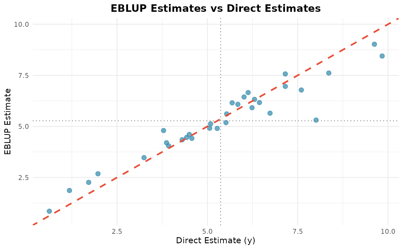
autoplot(fit_fh, type = "estimates")

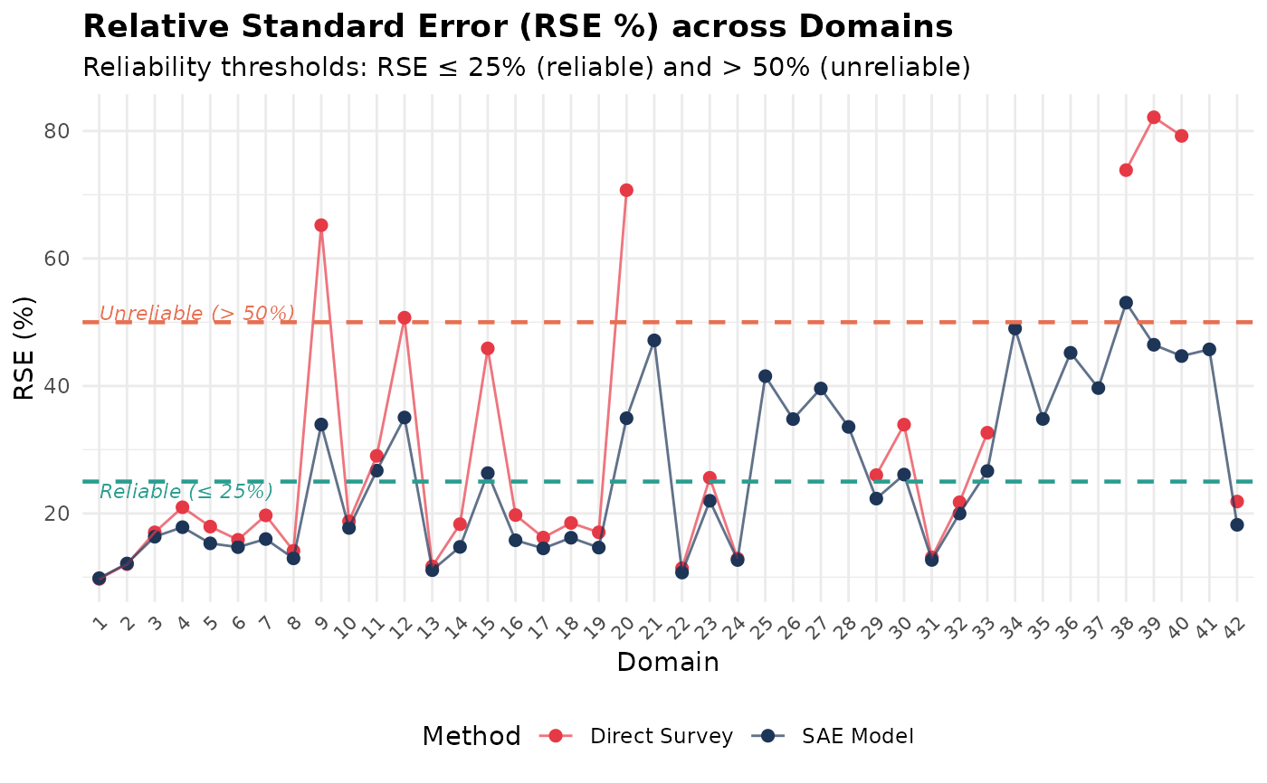
autoplot(fit_fh, type = "rse")
#> Warning: Removed 10 rows containing missing values or values outside the scale range
#> (`geom_point()`).


# Compare two models
fit_sfh <- eblup_sfh(y ~ x1 + x2 + x3, data = mys, vardir = "vardir", W = mys_proxmat)
#> 
#> ── Fast Small Area Estimation (fastsae) ────────────────────────────────────────
#> Call:
#> eblup_sfh(formula = y ~ x1 + x2 + x3, vardir = "vardir", data = mys, W =
#> mys_proxmat)
#> 
#> ✔ Convergence: Yes (in 18 iterations)
#> Model: Spatial Fay-Herriot (Area-level SAR)
#> Method: REML
#> Random effect variance (sigma2_u): 0.989226 
#> Spatial autocorrelation (rho): -1 
#> 
#> Fixed Effects Coefficients:
#>                   beta  std.error     zvalue pvalue
#> (Intercept)  3.2570714  0.6265689  5.1982651 0.0000
#> x1          -0.0020340  0.0080925 -0.2513457 0.8015
#> x2           0.0568516  0.0525488  1.0818827 0.2793
#> x3           0.0252179  0.0497283  0.5071123 0.6121
#> 
#> EBLUP Estimates (First 6 domains):
#>   domain        y    vardir    eblup random_effect       mse       rse
#> 1      1 8.359527 0.6618838 7.535193     2.8128506 0.4999462  9.383551
#> 2      2 7.599650 0.8374691 6.564385     2.2380505 0.5831410 11.633028
#> 3      3 5.514137 0.8822257 5.109460     0.7620572 0.6095214 15.279864
#> 4      4 3.869326 0.6581716 4.273391    -1.2736332 0.5018535 16.577378
#> 5      5 6.305063 1.2788021 6.791422     0.4746535 0.7644430 12.873951
#> 6      6 3.926807 0.3878004 4.016701    -0.9459807 0.3398919 14.514460
#> ... and 36 more rows.
#> 
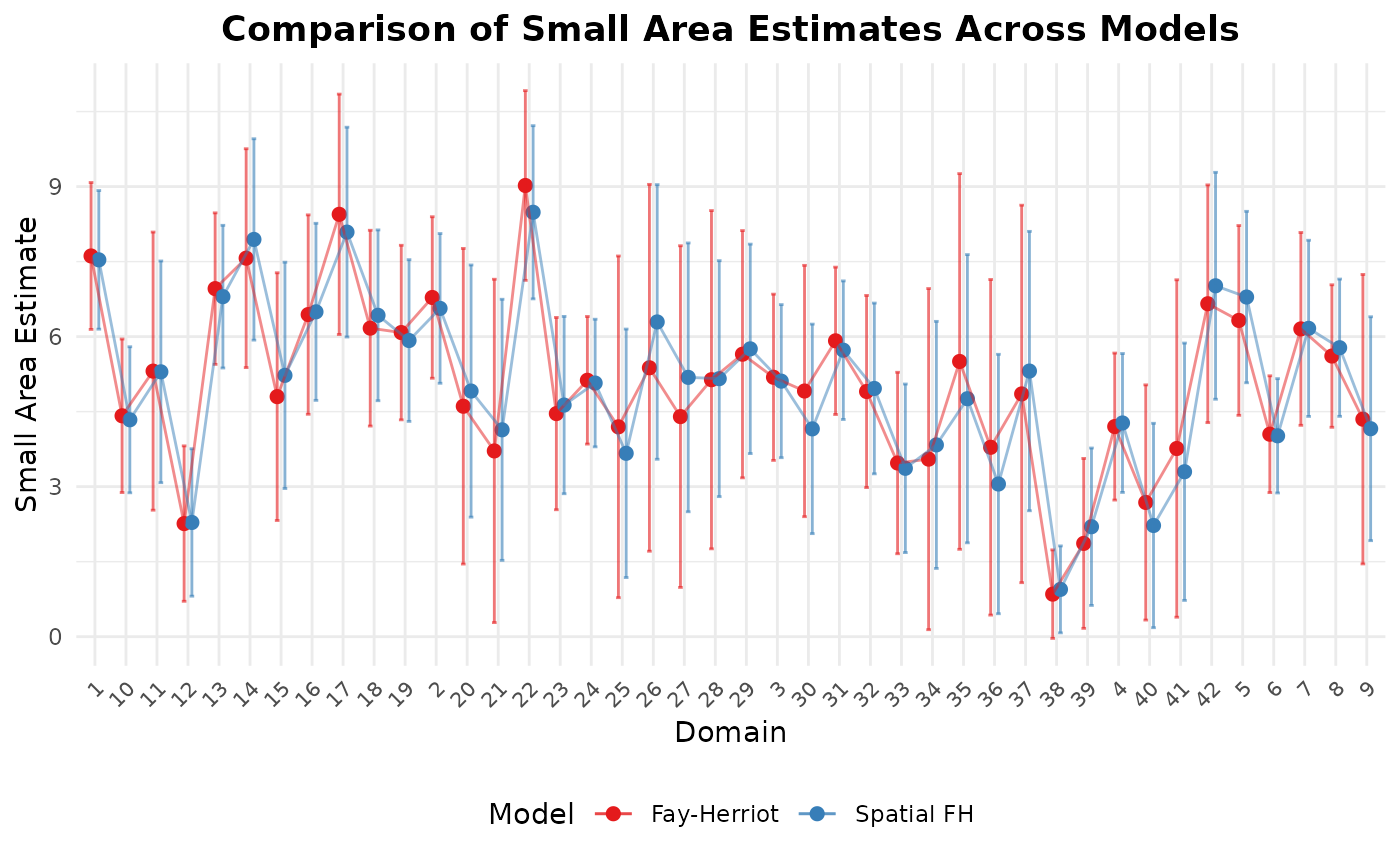
autoplot(list("Fay-Herriot" = fit_fh, "Spatial FH" = fit_sfh), type = "comparison")