Provides a comprehensive evaluation and concordance comparison between two fitted Small Area Estimation (SAE) models (e.g. comparing Classical Fay-Herriot vs Spatial Fay-Herriot, Area-level vs Unit-level BHF, or EBLUP vs HB).
Computes agreement, ranking and efficiency metrics:
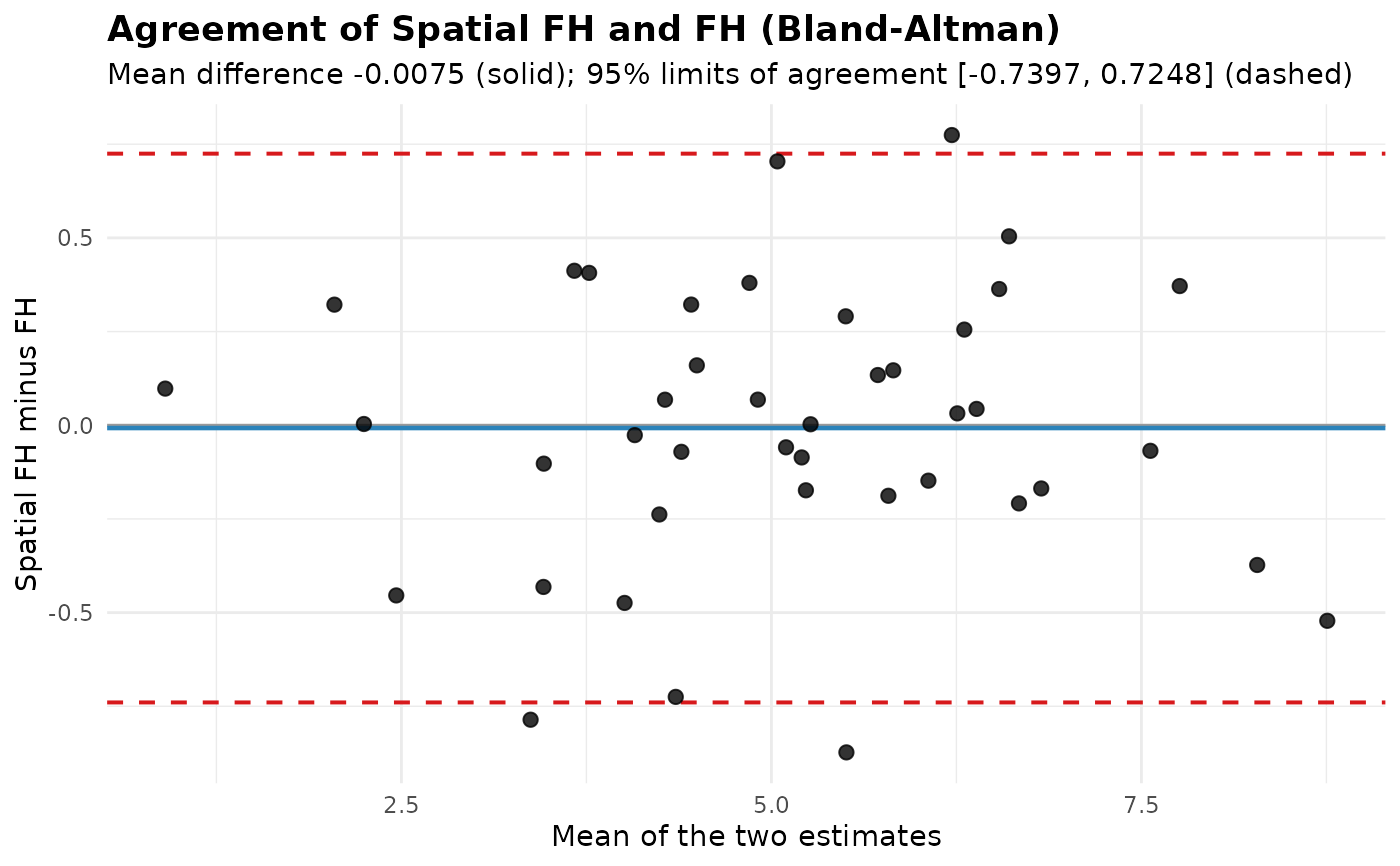
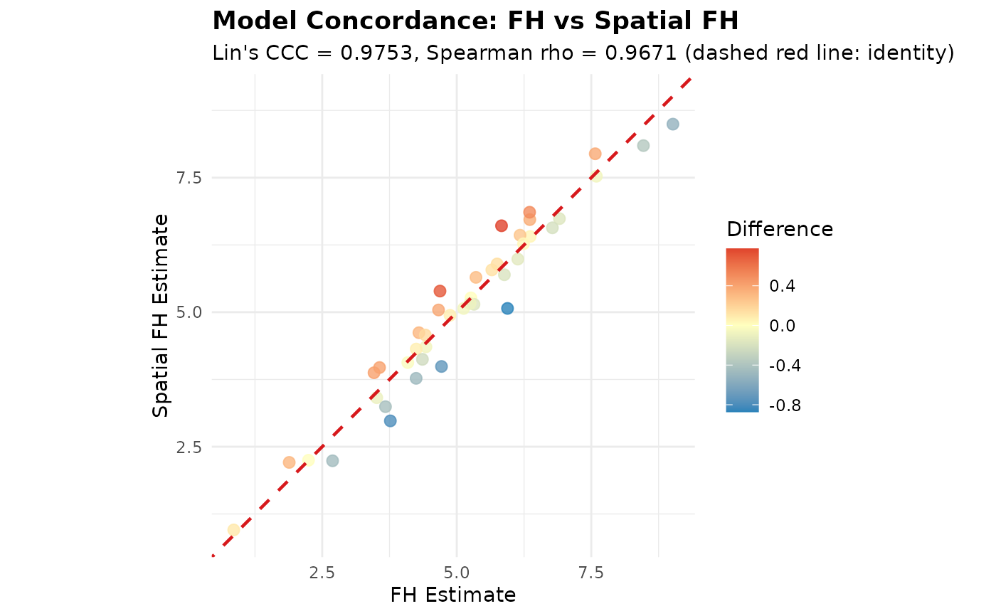
Agreement of the estimates (Bland and Altman 1986): the mean difference \(\bar d\) of Model 2 minus Model 1, the 95% limits of agreement \(\bar d \pm 1.96\, s_d\), the mean absolute difference (MAE) and the root mean squared difference (RMSD), and Lin's (1989) concordance correlation coefficient \(\rho_c = 2 s_{12} / (s_1^2 + s_2^2 + (\bar\theta_1 - \bar\theta_2)^2)\) (moments with divisor \(n\)), which is 1 only when the estimates lie on the identity line.
Differences relative to the uncertainty: \(z_d = (\hat\theta_{2d} - \hat\theta_{1d}) / \sqrt{\text{MSE}_{1d}}\), summarised by its median absolute value and the share of domains with \(|z_d| > 1\). This is descriptive, not a test: both estimators use the same data, so their difference has a smaller variance than either.
Ranking of the domains: Spearman's rank correlation, the mean absolute change of rank, and the share of the
tophighest and lowest domains of Model 1 that are also among the highest and lowest of Model 2 (the domains a programme would target).Efficiency: mean and median MSE ratio (\(\text{MSE}_1 / \text{MSE}_2\)), the share of domains where Model 2 has the lower MSE, and the mean RSE (%) of each model.
Pearson's correlation is not reported: two reasonable models of the same data correlate almost perfectly whatever their differences, and a correlation measures association, not agreement (a model that is 10% higher everywhere still has \(r = 1\); Bland and Altman 1986).
Usage
compare_sae(
  model1,
  model2 = NULL,
  names = NULL,
  thresholds = c(25, 50),
  top = 0.1,
  ...
)

# Default S3 method
compare_sae(
  model1,
  model2 = NULL,
  names = NULL,
  thresholds = c(25, 50),
  top = 0.1,
  ...
)

# S3 method for class 'fastsae_comparison'
print(x, ...)

# S3 method for class 'fastsae_comparison'
summary(object, ...)

# S3 method for class 'fastsae_comparison'
plot(x, y = NULL, ...)

# S3 method for class 'fastsae_comparison'
autoplot(
  object,
  type = c("scatter", "comparison", "difference", "mse", "rse"),
  title = NULL,
  ...
)
Arguments
- model1
A fitted
fastsaemodel object, or a list containing twofastsaemodels.- model2
A second fitted
fastsaemodel object. Ignored ifmodel1is a list.- names
Optional character vector of length 2 specifying descriptive labels for the models. Default is inferred from model types or call arguments.
- thresholds
Numeric vector of length 2 with the RSE (%) cut-offs drawn in
autoplot(type = "rse")(seeadd_reliability_flags). Defaultc(25, 50).- top
Share (below 1) or number (1 or more) of the highest and of the lowest domains whose overlap between the models is reported. Default
0.1(10%, at least one domain).- ...
Additional arguments.
- x
An object of class
fastsae_comparison(forprintandplotmethods).- object
An object of class
fastsae_comparison(forsummaryandautoplotmethods).- y
Ignored argument for compatibility with the generic
plotmethod.- type
Character string indicating comparison plot type:
"scatter","comparison","difference"(Bland-Altman plot: the difference against the mean of the two estimates, with the mean difference and the 95% limits of agreement),"mse", or"rse". Default is"scatter".- title
Optional character string specifying a custom plot title.
Value
An S3 object of class fastsae_comparison containing:
metrics: A data frame of the metrics above (columnsGroup,Metric,Value), formatted for printing.agreement: The same agreement, uncertainty and ranking metrics as a named numeric vector.data: A domain-level data frame with aligned estimates, MSE and RSE values, their differences, ranks (rank_1,rank_2,rank_change; 1 is the highest estimate) andz_diff.names: Vector of the two model names.thresholds: The RSE thresholds used.
References
Bland, J. M. and Altman, D. G. (1986). Statistical methods for assessing agreement between two methods of clinical measurement. The Lancet, 327(8476), 307-310.
Lin, L. I.-K. (1989). A concordance correlation coefficient to evaluate reproducibility. Biometrics, 45(1), 255-268.
Examples
library(fastsae)
data(mys)
# Fit two models
fit_fh <- eblup_fh(y ~ x1 + x2, vardir = "vardir", data = mys)
#>
#> ── Fast Small Area Estimation (fastsae) ────────────────────────────────────────
#> Call:
#> eblup_fh(formula = y ~ x1 + x2, vardir = "vardir", data = mys)
#>
#> ✔ Convergence: Yes (in 7 iterations)
#> Model: Fay-Herriot (Area-level)
#> Method: REML
#> Random effect variance (sigma2_u): 2.569182
#>
#> Fixed Effects Coefficients:
#> beta std.error zvalue pvalue
#> (Intercept) 3.0689476 0.7631917 4.0212018 0.0001
#> x1 -0.0041073 0.0090768 -0.4525074 0.6509
#> x2 0.0861173 0.0309576 2.7817847 0.0054
#>
#> EBLUP Estimates (First 6 domains):
#> domain y eblup vardir random_effect mse rse
#> 1 1 8.359527 7.594807 0.6618838 2.96835204 0.5602338 9.855256
#> 2 2 7.599650 6.777056 0.8374691 2.52354833 0.6766501 12.137828
#> 3 3 5.514137 5.247512 0.8822257 0.77645304 0.7048881 15.999508
#> 4 4 3.869326 4.247072 0.6581716 -1.47453645 0.5556741 17.551750
#> 5 5 6.305063 6.353632 1.2788021 -0.09757891 0.9308379 15.185005
#> 6 6 3.926807 4.090117 0.3878004 -1.08192989 0.3497100 14.458337
#> ... and 36 more rows.
#>
fit_sfh <- eblup_sfh(y ~ x1 + x2, vardir = "vardir", data = mys, W = mys_proxmat)
#>
#> ── Fast Small Area Estimation (fastsae) ────────────────────────────────────────
#> Call:
#> eblup_sfh(formula = y ~ x1 + x2, vardir = "vardir", data = mys, W =
#> mys_proxmat)
#>
#> ✔ Convergence: Yes (in 23 iterations)
#> Model: Spatial Fay-Herriot (Area-level SAR)
#> Method: REML
#> Random effect variance (sigma2_u): 0.980871
#> Spatial autocorrelation (rho): -1
#>
#> Fixed Effects Coefficients:
#> beta std.error zvalue pvalue
#> (Intercept) 3.1958831 0.6144952 5.2008269 0.0000
#> x1 -0.0035203 0.0075141 -0.4684949 0.6394
#> x2 0.0801807 0.0254664 3.1484875 0.0016
#>
#> EBLUP Estimates (First 6 domains):
#> domain y vardir eblup random_effect mse rse
#> 1 1 8.359527 0.6618838 7.526578 2.8428783 0.4976814 9.37299
#> 2 2 7.599650 0.8374691 6.568449 2.2426219 0.5795629 11.59011
#> 3 3 5.514137 0.8822257 5.161577 0.6429192 0.5946117 14.93944
#> 4 4 3.869326 0.6581716 4.315257 -1.3771626 0.4936622 16.28202
#> 5 5 6.305063 1.2788021 6.857796 0.4699659 0.7434759 12.57329
#> 6 6 3.926807 0.3878004 4.063760 -1.1194128 0.3305229 14.14727
#> ... and 36 more rows.
#>
# Compare models
comp <- compare_sae(fit_fh, fit_sfh, names = c("FH", "Spatial FH"))
print(comp)
#>
#> ── Small Area Estimation Model Concordance & Comparison ────────────────────────
#> Model 1: FH
#> Model 2: Spatial FH
#> Matched Domains: 42
#> ────────────────────────────────────────────────────────────────────────────────
#>
#> Agreement, Ranking & Efficiency Metrics:
#> Group Metric Value
#> Domains Matched Domains 42
#> Agreement Mean Difference (Spatial FH - FH) -0.0075
#> Agreement 95% Limits of Agreement [-0.7397, 0.7248]
#> Agreement Mean Absolute Difference (MAE) 0.2866
#> Agreement Root Mean Squared Difference (RMSD) 0.3692
#> Agreement Lin's Concordance Correlation (CCC) 0.9753
#> Uncertainty Median |Difference| / RMSE of FH 0.218
#> Uncertainty % of domains with |Difference| > RMSE of FH 0.0%
#> Ranking Spearman Rank Correlation (rho) 0.9671
#> Ranking Mean Absolute Rank Change 2.29
#> Ranking Shared Top 4 (highest estimates) 4 / 4
#> Ranking Shared Bottom 4 (lowest estimates) 4 / 4
#> Efficiency Mean MSE Ratio (FH / Spatial FH) 1.3758
#> Efficiency Median MSE Ratio (FH / Spatial FH) 1.2606
#> Efficiency % of domains where Spatial FH is more efficient 100.0%
#> Efficiency Mean RSE % (FH) 25.59%
#> Efficiency Mean RSE % (Spatial FH) 21.64%
#>
summary(comp)
#>
#> ── Small Area Estimation Model Concordance & Comparison ────────────────────────
#> Model 1: FH
#> Model 2: Spatial FH
#> Matched Domains: 42
#> ────────────────────────────────────────────────────────────────────────────────
#>
#> Agreement, Ranking & Efficiency Metrics:
#> Group Metric Value
#> Domains Matched Domains 42
#> Agreement Mean Difference (Spatial FH - FH) -0.0075
#> Agreement 95% Limits of Agreement [-0.7397, 0.7248]
#> Agreement Mean Absolute Difference (MAE) 0.2866
#> Agreement Root Mean Squared Difference (RMSD) 0.3692
#> Agreement Lin's Concordance Correlation (CCC) 0.9753
#> Uncertainty Median |Difference| / RMSE of FH 0.218
#> Uncertainty % of domains with |Difference| > RMSE of FH 0.0%
#> Ranking Spearman Rank Correlation (rho) 0.9671
#> Ranking Mean Absolute Rank Change 2.29
#> Ranking Shared Top 4 (highest estimates) 4 / 4
#> Ranking Shared Bottom 4 (lowest estimates) 4 / 4
#> Efficiency Mean MSE Ratio (FH / Spatial FH) 1.3758
#> Efficiency Median MSE Ratio (FH / Spatial FH) 1.2606
#> Efficiency % of domains where Spatial FH is more efficient 100.0%
#> Efficiency Mean RSE % (FH) 25.59%
#> Efficiency Mean RSE % (Spatial FH) 21.64%
#>
#> Distribution of Domain Point Estimates:
#> FH Spatial FH Difference
#> 0% 0.8555 0.9533 -0.8730
#> 25% 4.2455 4.0094 -0.1846
#> 50% 5.1879 5.1083 0.0030
#> 75% 6.1655 6.3740 0.2818
#> 100% 9.0169 8.4950 0.7744
#>
#> Distribution of Relative Standard Error (RSE %):
#> FH Spatial FH RSE Diff (1 - 2)
#> 0% 9.86 9.37 -1.98
#> 25% 14.83 13.52 0.76
#> 50% 21.85 18.23 2.20
#> 75% 34.76 26.03 6.15
#> 100% 52.75 46.45 17.39
#>
# Plot comparison
autoplot(comp, type = "scatter")
 autoplot(comp, type = "difference")